Chapter 15 Testing parts of models

require(mosaic) # mosaic operators and data used in this section

The basic software for hypothesis testing on parts of models involves the familiar lm() and summary() operators for generating the regression report and the anova() operator for generating an ANOVA report on a model.

15.1 ANOVA reports

The anova operator takes a model as an argument and produces the term-by term ANOVA report. To illustrate, consider this model of wages from the Current Population Survey data.

Cps <-  CPS85 # from mosaicData
mod1 <-  lm( wage ~ married + age + educ, data = Cps)
anova(mod1)

## Analysis of Variance Table
## 
## Response: wage
##            Df  Sum Sq Mean Sq  F value    Pr(>F)    
## married     1   142.4  142.40   6.7404  0.009687 ** 
## age         1   338.5  338.48  16.0215 7.156e-05 ***
## educ        1  2398.7 2398.72 113.5405 < 2.2e-16 ***
## Residuals 530 11197.1   21.13                       
## ---
## Signif. codes:  0 '***' 0.001 '**' 0.01 '*' 0.05 '.' 0.1 ' ' 1

Note the small p-value on the married term: 0.0097.

To change the order of the terms in the report, you can create a new model with the explanatory terms listed in a different order. For example, here’s the ANOVA on the same model, but with married last instead of first:

mod2 <- lm( wage ~ age + educ + married, data = Cps)
anova(mod2)

## Analysis of Variance Table
## 
## Response: wage
##            Df  Sum Sq Mean Sq  F value    Pr(>F)    
## age         1   440.8  440.84  20.8668  6.13e-06 ***
## educ        1  2402.7 2402.75 113.7310 < 2.2e-16 ***
## married     1    36.0   36.01   1.7046    0.1923    
## Residuals 530 11197.1   21.13                       
## ---
## Signif. codes:  0 '***' 0.001 '**' 0.01 '*' 0.05 '.' 0.1 ' ' 1

Now the p-value on married is large. This suggests that much of the variation in wage that is associated with married can also be accounted for by age and educ instead.

15.2 Non-Parametric Statistics

Consider the model of world-record swimming times plotted on page 116.

It shows pretty clearly the interaction between year and sex.

It’s easy to confirm that this interaction term is statistically significant:

Swim <-  SwimRecords  # in mosaicData
anova( lm( time ~ year * sex, data = Swim) )

## Analysis of Variance Table
## 
## Response: time
##           Df Sum Sq Mean Sq F value    Pr(>F)    
## year       1 3578.6  3578.6 324.738 < 2.2e-16 ***
## sex        1 1484.2  1484.2 134.688 < 2.2e-16 ***
## year:sex   1  296.7   296.7  26.922 2.826e-06 ***
## Residuals 58  639.2    11.0                      
## ---
## Signif. codes:  0 '***' 0.001 '**' 0.01 '*' 0.05 '.' 0.1 ' ' 1

The p-value on the interaction term is very small: \(2.8 \times10^{-6}\).

To check whether this result might be influenced by the shape of the distribution of the time or year data, you can conduct a non-parametric test. Simply take the rank of each quantitative variable:

mod <- lm( rank(time) ~ rank(year) * sex, data = Swim)
anova(mod)

## Analysis of Variance Table
## 
## Response: rank(time)
##                Df  Sum Sq Mean Sq   F value Pr(>F)    
## rank(year)      1 14320.5 14320.5 3755.7711 <2e-16 ***
## sex             1  5313.0  5313.0 1393.4135 <2e-16 ***
## rank(year):sex  1     0.9     0.9    0.2298 0.6335    
## Residuals      58   221.1     3.8                     
## ---
## Signif. codes:  0 '***' 0.001 '**' 0.01 '*' 0.05 '.' 0.1 ' ' 1

With the rank-transformed data, the p-value on the interaction term is much larger: no evidence for an interaction between year and sex. You can see this directly in a plot of the data after rank-transforming time:

xyplot( rank(time) ~ year, groups = sex, data = Swim)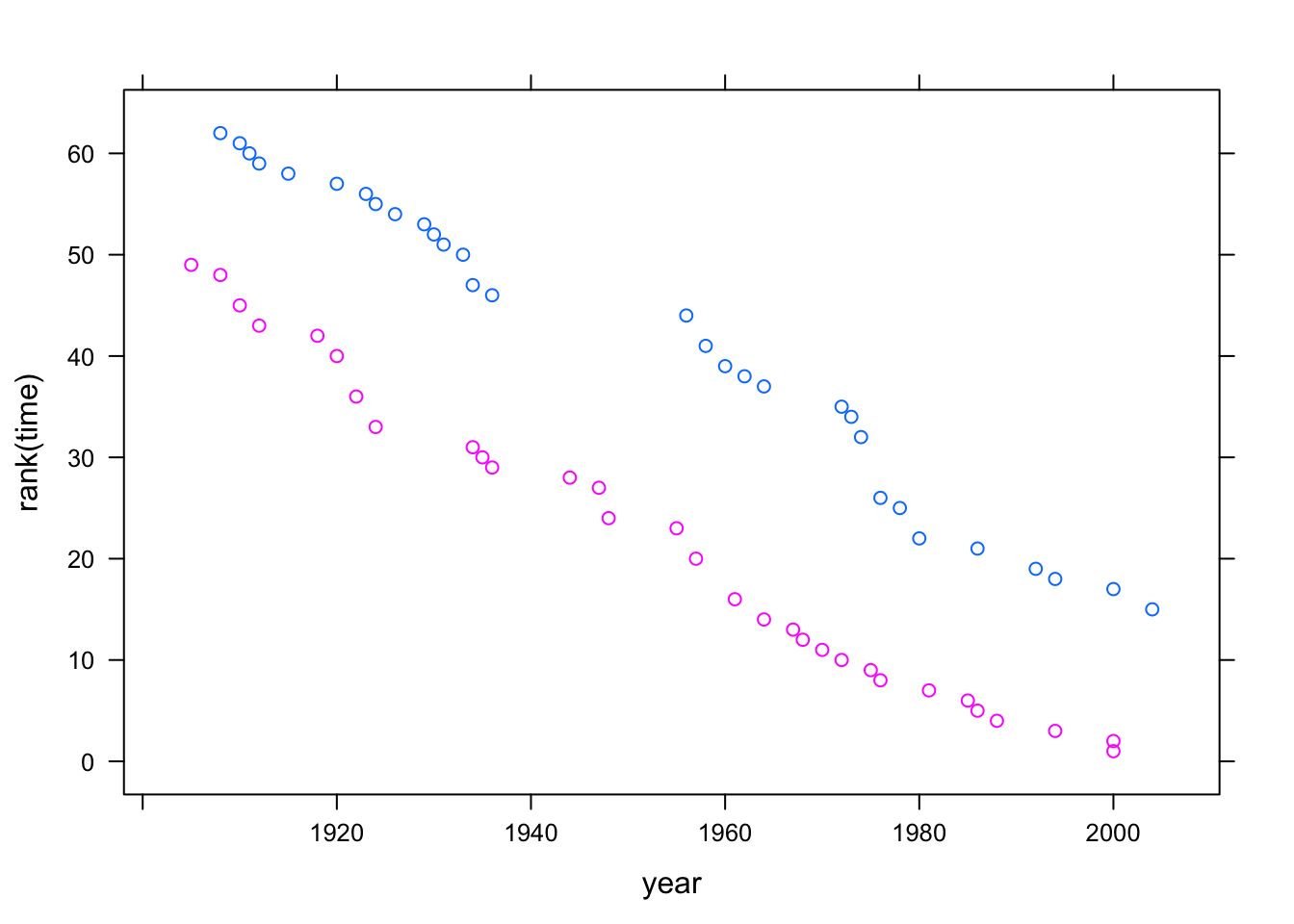

The rank-transformed data suggest that women’s records are improving in about the same way as men’s. That is, new records are set by women at a rate similar to the rate at which men set them.